A literature review:
The acoustics of the violin
Lei Fu April, 2015 Instructor: Prof. Gary P. Scavone
Final project of Seminar MUMT 618 Schulich School of Music, McGill University
5.2 Playabillity and transients
we have seen that the basic Helmholtz motion can only be altered in a rather subtle way, by varying the bow force to change the corner sharpness, or by moving the bowing point to vary the pattern of Schelleng ripples. It is time to stop pretending that violinists mainly produce steady tones: nothing could be further from the truth. Players are constantly ‘shaping’ each note as they play it.
How quickly, if at all, is the Helmholtz motion established after a given bow gesture? What does the terrain of transient length look like in parameter spaces relevant to a player?
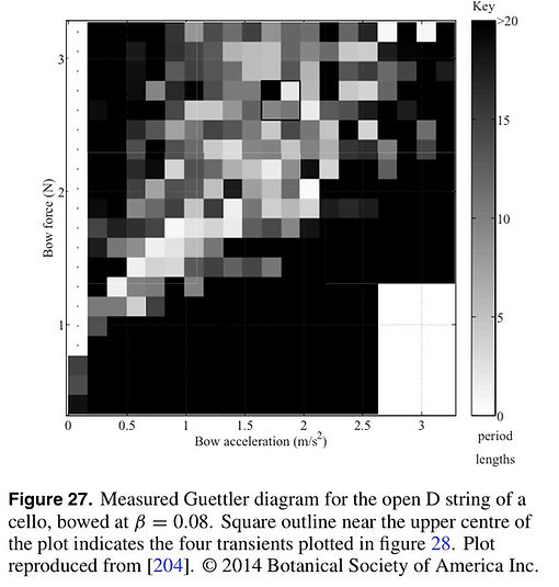
This realization led Guettler to study a particular two- dimensional family of transient gestures, leading to what has become known as a Guettler diagram. Guettler produced a prediction that ‘perfect transients’, in which Helmholtz-like motion is established from the very first slip of the string over the bow. figure 27 shows an example, measured on the open D3 string of a cello (147 Hz). Each pixel corresponds to a single constant-acceleration bow gesture. White for perfect transients, through to black for cases that still had not produced Helmholtz motion after 20 nominal period lengths.
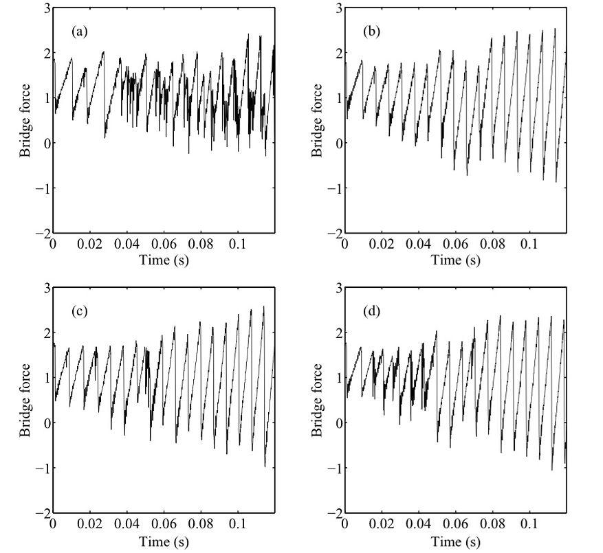
Figure 28 shows the block of four outlined by a square in figure 27.


If the friction-curve model is used, based on measured steady-sliding behaviour of rosin as plotted in figure 6, results are obtained as shown in figure 29(a). If instead a simple thermal-driven friction model is used (as introduced in section 2.4.2), calibrated against the same steady-sliding friction data, the result is as shown in figure 29(b). It is immediately clear that neither prediction matches the measurements very accurately, but that the thermal model comes a lot closer than the friction-curve model.

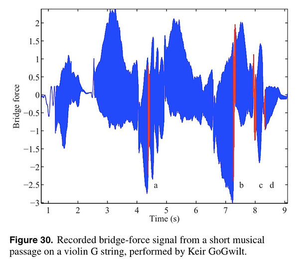
Figure 30 shows a few seconds of music, played by violinist Keir GoGwilt on the G string of a violin and recorded using a bridge-force sensor.
Four particular note transitions are highlighted in the plot, and shown in more detail in figure 31.
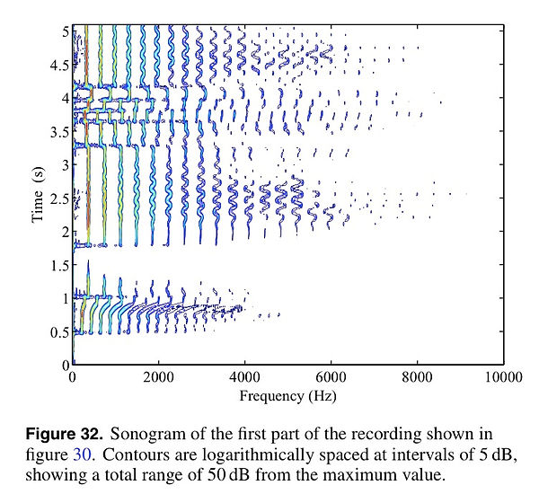
A different view of this same musical extract is given by figure 32, where the first half of the passage is shown as a time-frequency sonogram: the horizontal axis shows frequency and the vertical axis shows time, running upwards in the plot.