A literature review:
The acoustics of the violin
Lei Fu April, 2015 Instructor: Prof. Gary P. Scavone
Final project of Seminar MUMT 618 Schulich School of Music, McGill University
2.2 The first simulation models
As the computer arised, simulations started to be performed in the late 1970s. This allowed Cremer’s mechanism for the influence of bow force on tone quality to be investigated in quantitative detail. The most popular style of simulation can be described quite easily.
It is clearest to introduce the model methodology via the simplest case: assume that the motion of the string is confined to a single plane, the bow-hair is driven at a constant bow- speed vb, and the bow-string frictional contact occurs at a single point. Just two dynamical variables are then needed: the time-varying string velocity v(t) at the bowed point, and the frictional force f (t) at that point, as sketched in figure 5(a). These two variables are related in two different ways, indicated in figure 5(b). On the one hand, the force f is applied to a complicated linear system comprised of the string with its attached violin body, and familiar linear-systems theory can reveal the resulting response v. On the other hand, the two variables are related via a nonlinear constitutive relation characterizing dynamic friction at the contact. A closed feedback loop including these two effects results in self-excited vibration.
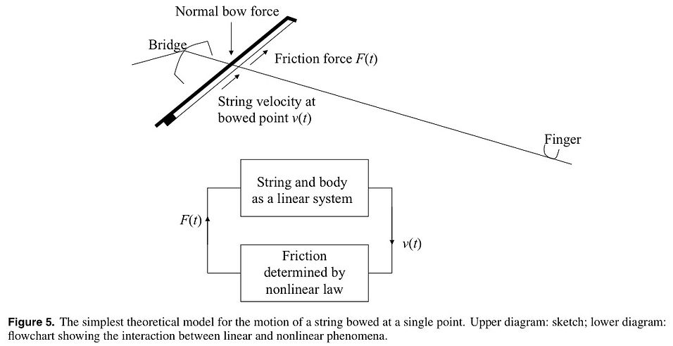


The string velocity at the bowed point associated with these waves should be well approximated by the ideal-string assumption, giving the simple proportional behaviour v = f/2Z0, (1) where is the characteristic wave impedance of a string with tension T and mass per unit length m.
The real string is not, of course, infinite. If the combined effect of returning waves from both ends of the string arriving at the bowed point at time t is a string velocity contribution vh (t ), then adding to equation (1) gives v=vh+f/2Z0 (2)The subscript h stands for ‘history’, because vh (t ) can be calculated from the past history of the motion as a result of the finite time delay.
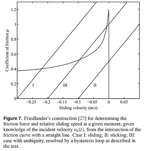
The nonlinear response of friction is a more difficult thing to characterize. It can be sketched in figure 6 and figure 7.

2.2.1 Helmholtz motion, higher types, and variation with bow
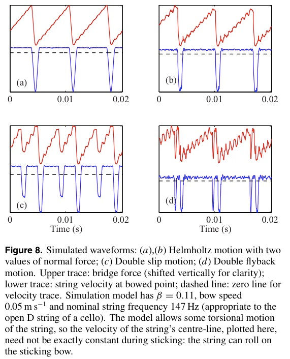
This model can indeed simulate Helmholtz motion and show the influence of bow force on the roundedness of the Helmholtz corner: examples are shown in figures 8(a) and (b). Each ramp of the sawtooth waveform is not a straight line as in the sketch of figure 2(c): instead, it shows a rather regular pattern of wiggles called ‘ripples’ by Schelleng and ‘secondary waves’ by Cremer . These ripples are caused by brief peaks in friction force during transitions between slipping and sticking, and their repeat time is associated with the wave travel time from the bow to the bridge and back.
Other waveforms from the same simulation model, simply varying the input parameters of bow force and position, are shown in figures 8(c) and (d). Figure 8(c) shows a typical waveform exhibiting two slips per cycle instead of one, the result of a bow force just below the Schelleng minimum value. Figure 8(d) shows a rather different periodic waveform, usually called ‘double flyback motion’ .
2.2.2 The flattening effect
when the straight line intersects the friction curve in three points rather than one, what should be done? The result is hysteresis: when vh(t) increases through the ambiguous range the string continues to slip as long as possible, but when it decreases through the range it continues to stick as long as possible. The middle intersection of any group of three is unstable and is never chosen.
The scope for flattening is determined by how rounded the Helmholtz corner is: each stick-slip transition must occur somewhere within the range of the rounded corner, and so the corner width puts a limit on the possible extent of flattening.
2.2.3 The effect of finite bow width
In the simple form of simulation model introduced so far, the bow-string contact has been assumed to occur at a single point. This is obviously unrealistic: the ribbon of bow hair is several millimetres wide.
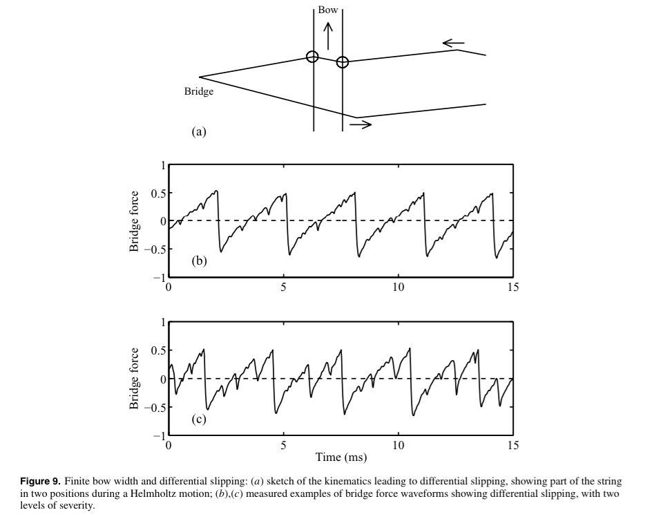
The most important effect can be explained by a simple kinematic argument, illustrated in figure 9(a). The portion of string in this contact region would be transported by the bow motion in a parallel manner. This parallel motion would lead to kinks in the string at the edges of the bow, requiring concentrations of friction force to maintain the state of sticking. These may prove impossible without exceeding the limit of sticking friction, and the result is that the string slips over some, but not all, of the bow-hairs near one or both edges to relieve the stress. This ‘differential slipping’ may occur in a regular or an irregular way.
Two typical measured examples of the resulting bridge force waveform are shown in figure 9(b), exhibiting differential slipping with different degrees of severity. To a listener the result is a component of ‘noise’ accompanying the musical note, which grows with the severity of the differential slips. A skilled player can control this level of noise from differential slipping.
2.2.4 The wolf note
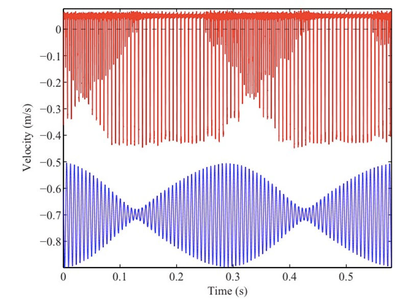
For losses associated with wave reflection at a non-rigid termination, the more the body moves the greater is the energy dissipation rate, and the higher the resulting minimum bow force. Now consider what happens when starting to bow a note matching a strong body resonance. Initially the body is not vibrating, and it may be possible to start the Helmholtz motion with a relatively low bow force. The resonant response of the body will then grow, with a timescale determined by the damping factor of the mode in question. This causes the bridge motion to increase, so the effective minimum bow force rises. If the player maintains the low initial bow force, it may happen that the minimum level overtakes the actual bow force. Helmholtz motion then gives way to double-slipping motion. But such motion, especially if the two slips are rather symmetrical, produces far less excitation at the fundamental frequency, and this allows the body vibration to die away. The effective minimum bow force may fall below the actual force, and Helmholtz motion may be able to re-establish. The cycle then repeats, and the result is the ‘warbling wolf’.
In figure 10, the bridge force waveform shows alternation between Helmholtz motion and double- slipping motion. The body motion is also shown, and the phase relation between it and the string oscillation regime bears out the description just given: Helmholtz motion breaks down when the body motion becomes too large, and resumes when it becomes sufficiently small.